The Excel Financial period formula is a calculation that’s worth keeping in your pocket. A lot of companies work this way and knowing the Excel financial period formula is a great way of comparing values across even date periods. What does that mean?
Well say if you wanted to compare sales between two months, maybe February and March. The trouble is that, presuming it’s not a leap year, February has 28 days and March 31 days. So it’s unfair to compare the two.
Hence you can split your calendar into financial periods so that when you company Period 2 with Period 4, you are comparing like for like.
How to create a financial period formula in Excel?
Here’s how to create a financial period formula in Excel. Do the following:
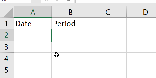
- Open a blank Excel spreadsheet.
- Add the column headers Date and Period in cells A1 and B1.
- Enter a Date in cell A2.
- In cell B2 enter the formula:
=MATCH(A2-DATE(YEAR(A2),1,1)+1,{1,31,61,91,121,151,181,211,241,271,301,331,361},1)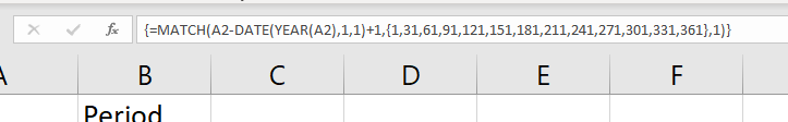
- Hold down Ctrl & Shift on the keyboard then press enter. (This is an array formula if you’re using later versions of Excel you don’t have to hold down Ctrl & Shift).
- Enter more dates and autofill so you can see the results.
How does this financial period formula work?
So now I bet you’re wondering how this formula works so let’s break it down.
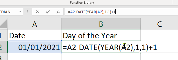
First, let’s look at the inner part of the function. That’s the A2-DATE(YEAR(A2),1,1)+1, what does this part do? Well, it returns the day of the day. Give it a go in a spreadsheet. Type in any date, on a blank spreadsheet, and then point this formula to it.
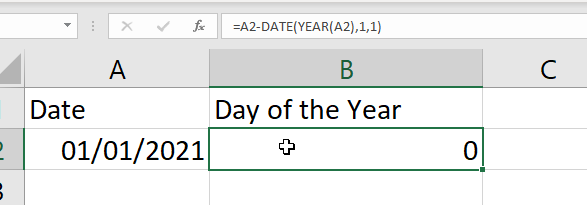
If you are still scratching your head over this calculation then basically it subtracts the date in question, A2, from the start of the current year. We then have to add one to the value to give the accurate date. If you truly want to see why we need to add 1, then enter the 1st of January of the current year in cell A2 and remove the “+1” part of the formula. You will see the number 0.
Great, so now that understand what that part of the formula is doing, next with have to introduce the MATCH function. So what is the purpose of the MATCH function?
You many have used the MATCH function with INDEX MATCH. Yes, it’s the same function! However, this time we’re going to enter in the values ourselves instead of referring to list. So what are all of these values we are entering?
Why use 13 Financial Periods?
As mentioned before, to compare figures it’s best done on an even platform. Basically, you cannot compare sales in February with sales in March. It’s not fair, as the number of days are not the same. It’s like them both running a 100m race and having March start 8.5 metres ahead of February. That’s simply not cricket my friend. Therefore we translate all dates in the year to a specific 30 day period.
So those numbers 1,31,61 etc. are effectively adding 30 onto each day. 1 add 30 is 31, 31 add 30 is 61 and so on until you reach the end of the year, which is 361. Yes, I can hear you say, that does mean that the last period has an extra four days. But nothing is perfect. So companies include those days in the 13th period, some carry it over to another year and some have a 14th period. However, I find that option to be rarely done.
What are the Curly braces in the financial period formula?
Right then! With me so far? What are the curly braces in the financial period formula? The braces turn the formula into an array formula. What does that mean? Think of it this way.
Array formulas
When you used the MATCH function in conjunction with INDEX, remember the INDEX MATCH function we looked at earlier? We referred to a list of cells. In other words the formula would look something like this:
=MATCH(A2,K2:K34,1)
The 2nd argument in the formula would be a list of cells that the MATCH function would be trying to match the value in A2 against. Now remember that in this above function we’re not referring to a list of cells we are typing them in manually.
In that case we need to tell Excel that the range that we are cross referencing isn’t a range of cells but an array, in other words a list. Let’s put it this way if we tried to type the following formula into an Excel sheet:

We would get this error:
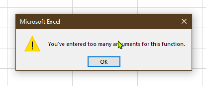
This is because the MATCH function is looking for 3 arguments, and here we have loads. So what do we do? We encase the numbers that we want to use as the array in braces, like this:
=MATCH(31,{1,31,61,91,121,151,181,211,241,271,301,331,361},1)
The simple action of placing braces (curly brackets) around the numbers in the second argument in the MATCH function, allows the MATCH function to view the numbers as one “Array”, or one list. When you press enter in this function it returns the number 2 as 31 is the second it the list. (If you’re using an older version of Excel you will have to hold down Ctrl & Shift when pressing enter).
Change the number in the first argument of the MATCH function, this represents the day of the year. Remember we worked that formula out earlier. When we enter in 75 for example, which would equate to the 16th of March in date terms, we get the number 3. This is because 75 is between 61 and 91 and so the MATCH function selects 61 as it’s the third number in the list. Now why does the MATCH function do that instead of select the 91. This is all down to the last argument in the MATCH function.
MATCH function MATCH Type Argument
Notice that in our formula, in the last argument of the MATCH function we entered the number 1.
=MATCH(75,{1,31,61,91,121,151,181,211,241,271,301,331,361},1)
What’s purpose of entering the number 1 at the end? Well, when you are typing in the MATCH function you may have noticed that you can type in one of 3 values as the last argument of the MATCH Function, which is the match type.
If you look on the Microsoft support page for the Match function it explains that the last argument, the match type argument, specifies how Excel matches the lookup value with values in the array. We have entered the number 1 which means that MATCH finds the largest value that is less than or equal to the lookup value. What does that mean? Have a look at the following:
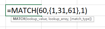
As you can see we’ve added a one in this simplified formula. Note that the final argument is 1 which means that when the MATCH function is looking along the array it knows that the number 60 is between 31 and 61. It selects the 31, or the second item in the list, because 31 is less that or equal to 60, it couldn’t choose 61, because 61 is greater than 60.
If we enter a -1 instead of 1 in the final argument, then the number returned is #N/A. This is because the list of days are in the wrong order. If you look again on the Microsoft support page you can see that if we use “-1” then our array list must be placed in descending order. In other words if we wanted our financial period formula to work using a “-1” we would need to arrange the list like this:
=13-MATCH(D2-DATE(YEAR(D2),1,1)+2,{361,331,301,271,241,211,181,151,121,91,61,31,1},-1)
As you can see we’ve had to make a little adjustment to the formula, as now the formula is looking in reverse. But there’s no need to go through all of that. Also, the final argument in the MATCH function can be a 0 if you want to find an exact match. This would not work in our example due to the fact that the day might not exactly the same as an item it the list.
13 Periods of 28 Days
If you wanted to create 13 periods of 28 days each to give the periods a more even split you could do the following:
=MATCH(A2-DATE(YEAR(A2),1,1),{0,28,56,84,112,140,168,196,224,252,280,308,336,364},1)
Because I haven’t added a one to the lookup value argument in the MATCH function I have to start the periods from Zero.
But if you wanted proof it takes into account all 13 periods then enter the following formula:
=MATCH(A2-DATE(YEAR(A2),1,1)+1,{1,29,57,85,113,141,169,197,225,253,281,309,337,365},1)
As you can see the last number in the Array is 365. Hence, the years are split into 13 even periods. However, this again isn’t perfect as it doesn’t take into account leap years. If you have any idea of how to do that then please stick the answer in the comments.
Financial Period Conclusion
Phew! That’s it! – Now I know this isn’t perfect, but I hope that this explanation goes a long way into explaining how to create a financial period formula in Excel.
I’m still learning about this so if you have any comments, stick them down below.
Also, here’s the financial period file that I’ve been working with. I haven’t tidied it up but maybe it’s of help to you.