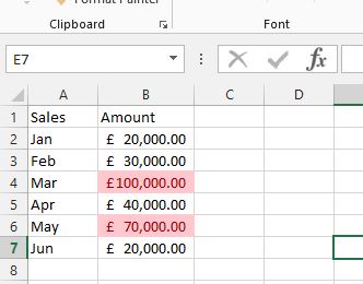

You want to change the colour of multiple cells based on the cells value then this is how you do it. In the following exercise you will change any number above £50,000 to red.
You can, of course, use conditional formatting to change the colour of a cell based on a numerical value. However you can also change the colour of multiple cells depending on many other factors.
Conditional Formatting based on another cells value
Conditional Formatting
Excel version (2007 – 2016)
- Open up a blank workbook and click in Cell A1.
- Enter the following information:
SalesAmountJan20000Feb30000Mar100000Apr40000May70000Jun20000 - Format the numbers as currency. (Just so it looks nice and tidy).
- Highlight all of the currency figures.
- Click on the Home tab then on Conditional Formatting to the right.
- Go down to Highlight Cell Rules then click Greater than.
- In the Greater Than box that appears enter 50000 in the greater than box.
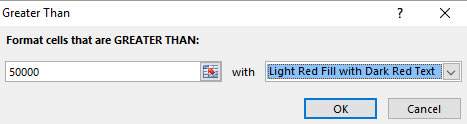
- Click OK.
- Note that all the numbers above £50,000 are now red.